Program Architecture
The simulations and graphs referenced earlier are produced with a computer program named eSim2 (election simulator, version 21). The program’s architecture and capabilities are described here.
Political Design
The program reads one or more configuration files, each of which contains a design. A design specifies how the political unites are organized for an election. For example, that in a FPTP election all the ridings elect one MP but that in an STV election a (larger) riding elects several.
Each design starts with existing real-world ridings from some real-world election:
- 1 or more real-world ridings are grouped into a virtual riding. A virtual riding may be the same as a real-world riding (when simulating FPTP or AV elections) or several (an STV and other scenarios). A real-world riding may be split between multiple virtual ridings, assigning a percentage to each.
- 1 or more virtual ridings are grouped into a region, each with zero or more top-up MPs. This comes into play in compensatory designs like Mixed Member Proportional or Rural-Urban Proportional. In many designs (including FPTP) each region contains exactly one virtual riding.
- 1 or more regions are grouped into a province. This is important in Canada where we have a constitutional requirement that the provincial results are independent of each other.
This is shown visually in Figure 1.
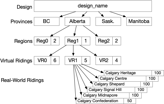
Figure 1: Visualizing a design
The design consists of four provinces (due to space on the page!). Alberta is divided into three regions. Reg1 has 1 top-up MP while the other two have 2 each. Reg1 has three virtual ridings and a total of 6+5+4 = 15 MPs to elect. Five of those MPs will be elected in virtual riding 1.
Virtual riding 1 is composed from six real-world ridings. Five of those are included completely in VR1. One of them, Calgary Confederation, is split 50-50 between this virtual riding and one or more others (not shown).
Common designs include:
- FPTP: Each province has one region with zero top-up seats; each region has one virtual riding that elects one MP; each virtual riding has one real-world riding.
- STV: Each province has one region with zero top-up seats;
each region has one virtual riding that elects n MPs;
each virtual riding has a number of real-world ridings, probably n of them. - MMP: Each province has one or more regions, each with one or more top-up seats;
each region has multiple virtual riding that each elect one MP;
each virtual riding has one to a small number of real-world ridings, possibly combined to generate the seats used for the top-up seats. - Rural-Urban: Similar to MMP but with virtual ridings electing 1 or more MPs.
- List: Similar to STV but with a different counting algorithm.
The design also carries information about:
- which elections it is applicable to (a design with 308 ridings is applicable to the 2006, 2008, and 2011 federal elections but not 2015 or 2019).
- which vote counting algorithms are applicable.
- which ballot generators are applicable.
- which representation equity utility functions to use.
- a list of optional transformations.
For the technically inclined, the design is stored in a super-set of JSON.
The Pipeline
Each design goes through a pipeline that ultimately produces the simulations and associated data. The pipeline may branch, so that one design potentially results in several simulations. The pseudocode is as follows:
forEach design, d:
  forEach applicable election, e:
    d1 = read the real-world candidates for e and add them to d
    d2 = d1 with optional transformations applied
    forEach applicable ballot generator, b:
      d3 = d2 with ballots for each candidate
      forEach vote counting algorithm, vc
        r = results of running vc on d3
        write web pages with r
          forEach repEffectivenessScore definition, res
            create appropriate graphs and stats
Transformations
There are a set of optional transformations that may be applied to a design. The transformations that have been defined so far and are actively used include:
- IncludeProvinces: This transformation includes only specified provinces.
Before the program was optimized to run faster, this was a crucial step in getting a fast enough turnaround time to make debugging practical. - CandidateConsolidation: Simply combining all the real-world candidates for a Canadidan election into an STV-like design results in many more candidates than would actually run. This transformation estimates how many candidates would run consolidates real-world candidates into that number.
Future work will likely use a transformation to perturb real-world elections. That allows us to see what happens with various systems if increasingly large percentages of voters defect from one party to another (the basis for my “swing analysis” as described on page 4 of my written testimony to the Electoral Reform Committee).
Transformations could also be used to manipulate the number of voters in each riding to measure how variation affects the Representation Equity Index.
Currently, transformations are only applied early in the pipeline to the design and candidates. There is a second class of transformations that could, in principle, be applied after ballots are generated.
Ballot Generators
So far there are two ballot generators defined, one for single-member plurality and one to generate ranked ballots.
Future work will likely involve different ballot generators. Exploring the Representation Equity Index for real-world STV elections, for example, would “generate” the ballots by reading data from a file.
Many others have used an n-dimensional space to describe the positions of candidates and voters with a voters’ ranking of each candidate defined by the Euclidian distance between them. Incorporating this into the program would involve implementing a new ballot generator.
Ballots are represented as a vector of candidates in preference order, the candidate under current consideration, the number of voters who voted this way (to avoid duplicating otherwise identical ballots), and the weight the ballot carries (for systems that transfer votes).
Vote Counting Algorithms
A vote counting algorithm is responsible for counting the votes (ballots, actually) to determine the elected and not elected candidates for the election.
So far, three have been implemented:
- Single Member Plurality: The one candidate with the most votes wins.
- Alternative Vote: Until a candidate has at least 50%+1 votes, drop the candidate with the least votes and transfer those ballots to the next preferred candidates.
- Single Transferable Vote: The current implementation uses the
Droop quota
with the
Gregory method. It’s built with a framework for implementing a
family of STV algorithms that permits easy variations in
- calculating the quota
- determining the trailing candidate to eliminate
- transfering all votes from an eliminated candidate to other candidates
- transfering surplus votes from a winning candidate to other candidates
Further counting algorithms need to be implemented for list PR schemes.
Counting algorithms for MMP and Rural-Urban Proportional will likely combine these more basic algorithms.
Representation Effectiveness Utility Functions
Finally, the results of each simulated election at the end of this pipeline is evaluated with a function that assigns a “representation effectiveness” value of the outcome to each voter. This is described much more completely in the Methodology section
There are currently two different functions implemented, one of which takes parameters and is used twice in the currently published results.
Top n preferences
This follows the description in the methodology
section closely. n is a parameter to the function.
Let j be the minimum of n and the number of
preferences expressed by the voter. The first preference has a weight of 1.
Each subsequent preference has a weight that is decreased by 1/j. Sum
up the weights of all those candidates that were elected.
For example, suppose n is 6 and that a voter’s ballot lists [A, B, C, D, E, F, G, H] as their preferences and that B, C and E were elected. Then the voter’s representation effectiveness scores is 0+(1-1/6)+(1-2/6)+0+0+(1-5/6) = 10/6. Recall that these scores are then normalized so that the average is 1.
Similarly, if n is again 6 but the voter’s ballot lists [B, A] as the preferences and A was elected, then their score is 0+(1-1/2) = 1/2.
The currently published results use this function with _n_=1 and _n_=6.
Voted for an elected candidate
This utility function assigns the value of 1 if any of the voters’ preferences were elected and 0 otherwise.
-
It’s the second public version; about the 8th internal version! ↩︎